Working with LTV and retention curves

Ivan Ignatov

Problem statement

Most of the analytical tasks in the field of user Acquisition for gaming applications, as well as tasks related to economic calculations in game design, are somehow based on knowledge of the key indicators of the project – the retention curve and the LTV curve.

The retention curve r(t) is a function reflecting the dependence of the proportion of users remaining in the project on the time that has elapsed since their registration. For example, if 10.7% of users remain in the project on the 7th day after registration, and 8.8% on the 10th day, then they say that retention is 0.107 and 0.088, respectively. That is, r(7) = 0.107, r(10) = 0.088.

The LTV – L(t) curve is a function reflecting the average income per player depending on the time since registration. For example, if users bring in an average of $2.55 per month from the moment of registration, then they say that “LTV 30 is 2.55”. That is, L (30) = 2.55.

Often, the abbreviation LTV is not the function L(t) itself, but the value of income “for the entire lifetime of the user”, that is, L(∞). Since this value can only be known for very long-standing applications for which it is too late to do analysis, in practice they often operate with an average income for six months or a year, that is, values of L(182) or L(365). For example, the phrase “traffic should pay off in six months” means the requirement of L(182) ≥ CPI.

In many cases, it is necessary to construct an analytical expression r(t) or L(t), that is, to “write a formula” for the curve, based on the available project statistics. Or, mathematically speaking, to approximate the statistical data of an analytical curve.

Examples of such tasks can be:

• prediction of retention and LTV for several months ahead for a project that has not yet reached the appropriate age;
• LT (Lifetime) rating of the average user;
• evaluation of the payback of advertising traffic based on the results of the first days after the start of the advertising campaign;
• the game designer builds such a scale of experience by levels so that there are approximately the same number of players at all levels;

Approach to the task from the right side

When an analyst is faced with the need to build such a formula, or at least with a choice of models available on the Internet, it is useful to keep in mind the following.

There are many banal truths that each of us is aware of, for example, such as “all users will leave the project sooner or later”, “the average user’s lifetime cannot be infinite”, “the more time has passed since registration, the smaller the proportion of remaining users” or even the obvious “at the time of registration, each user active.”

But not every formula, not every model used to approximate r(t) or L(t), stands up to the test of compliance with these “banal truths”.

For example, hyperbole is sometimes used as a retention model:

When C > 0, it gives a significant group of users who never quit the application.

As an LTV model, the so-called “power trend” L(t) = At ^B is also sometimes used, which simply assumes an infinite LTV, if we consider it “for the entire lifetime of the user”.

This leads to the fact that often the chosen model cannot approximate the available data well enough, or it can in the available time interval, but it begins to “fool” when it is “asked” to make a forecast for several months ahead.

Next, I describe an approach to “writing a formula” based on the study of the natural properties of the desired functions. Its essence is to choose from the whole variety of possible formulas exactly those whose properties coincide in advance with our empirical ideas about the behavior of the project audience. And not only the simplest ideas, “banal truths”, but also more complex ones. In particular, such as “the longer the user is in the project, the less chance that he will leave it today.”

The relationship between retension and LTV

Before solving the problem directly, it should be noted that the search for the type of LTV curve can be reduced to the search for the type of curve for the retention, that is, instead of two different tasks, consider one. This is done as follows.

The time derivative L`(t) of LTV makes sense of the accumulated income from the average user per unit of time and is inherently close to the retention curve r(t). Moreover, with a constant income per unit of time from a live player, they are simply proportional to each other: L`(t) = A r(t).

The value of A in marketing is usually called ARPU (Average revenue per user, average revenue per user). Unfortunately, ARPU is often understood to mean something else. For example, L(30) is often called “ARPU of the first month”. But as part of our work, we will understand by ARPU exactly the average amount of income from a live player per unit of time, and nothing else.

Often, in the first approximation, A is assumed to be constant, independent of the age of the user, which means L`(t) and r(t) changing according to the same law. In practice, it turns out that this is not the case – in particular, non-paying users quit the game on average earlier than paying ones, and therefore A grows depending on how many users are already playing, that is, from t. In other words, A = A(t) and L`(t) = A(t) r(t).

However, even in this case, A(t) remains quasi-constant, slowly changing in comparison with L`(t) and r(t), and this gives grounds to look for formulas for their changes in the same family of curves.

This approach is applied, and its validity is confirmed in practice by the fact that the resulting smoothed L(t) are quite close to the original empirical LTV curves of the projects under consideration.

Output of the desired curves

So, we will output r(t). What laws, what “natural properties” is this process subject to?

To begin with, we will write out those properties that we have referred to as “banal truths” above:

1) r(0) = 100% = 1 (all users are alive at the time of registration)
2) r(t) decreases by [0 ; ∞) (on average, users leave the game)
3) ∫₀^∞ r(t) dt is finite.

What does it mean, “the integral is finite”?

Let’s say a stable project receives incoming stable traffic at a rate of N people per unit of time (per day).

Then in the project of players with an age from t to t+h, N r(t) h will be obtained, and the total number of living players in the project will be the sum of all these values along the entire axis of the player’s age in increments of h, that is:

From practice, we know that even with an arbitrarily long, uniform pumping of the project with traffic, its live audience does not grow indefinitely, but reaches a kind of permanent “plateau”, and to overcome this plateau, more traffic is needed, that is, to increase N. Hence, M is finite, and, accordingly, the integral under consideration is finite.

By the way, from here on the fingers it can be seen that the average user’s lifetime:

This statement can be confirmed by more rigorous calculations, based on the concept of expectation and the fact that the density f(t) of the distribution of players over the lifetime in the project is determined by the equality f(t) = -r’(t).

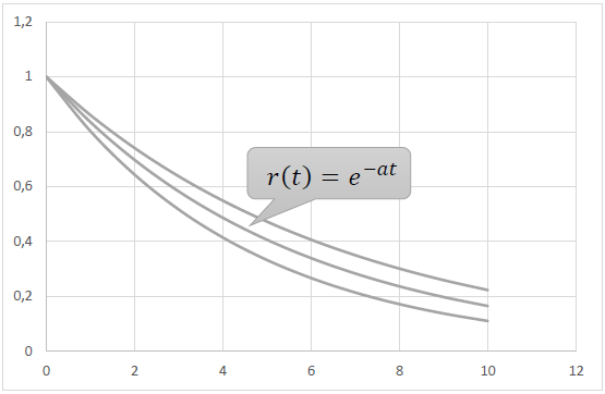
Properties 1) – 3) are satisfied by the simplest elementary function r(t) = e^-at, a > 0.

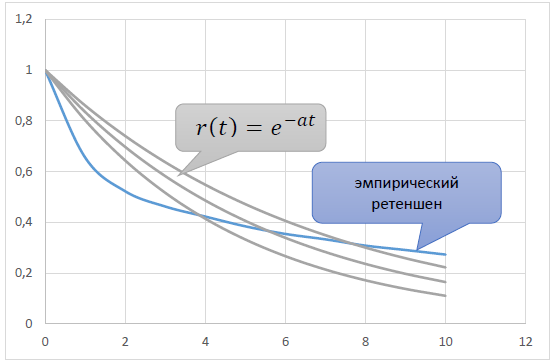
However, when trying to use the functions of this family, we encounter the following picture. The real empirical retention decreases faster at the beginning of the age axis than e^−at, and then slower.

What does this mean? That in the beginning, shortly after registration, players run from the project faster than according to the law r(t) = e^−at, and then, after being in the game for several months, slower.

This behavior is explained by the following empirical property of retention:

4) The longer the time since registration t, the less the “probability of outflow” p(t) .

The “churn probability” is the probability that the user will leave the game for the next unit of time, provided that he has not done this before.

How are p(t) and r(t) related?

Suppose we have an input traffic flow of N players per unit of time, then N r(t) players lived to age t, N r(t+h) players lived to age t+h.

Consequently, in the age range [t ; t+h], N r(t)− N r(t+h) players out of N r(t) available are lost. So, in h time, the project leaves the share of players equal to

It should be emphasized that the time here is understood as the subjective time of the players that has passed since their registration, and not some objective time interval common to all. Then, for a unit of time, the project leaves the share of players equal to

Since this fraction is equal to the considered probability, then:

Let’s go back to rule of thumb 4), according to which p(t) decreases and see how it holds for the law r(t) = ^e-at.

That is, the model p(t) is constant, not decreasing. That is why there is such a discrepancy between empirical r(t) and model r(t)=e^-αt.

Let’s try to generalize the model so that p(t) decreases.

Take p(t) = at ^β

• For β = 0, we obtain the already considered model p(t) = α , r(t) = ^e-at
• At β < 0 we get the decreasing probability of outflow we need.
• At β > 0, we get some strange application with the probability of outflow increasing as the player lives. For example, a game with strictly time-limited content.

Based on the new model:

If β ≠ -1, then

In this case, r(0) = 1, hence e ^C = 1, that is:

Having reassigned β+1 = b, α/(β+1) = a, we obtain the retention model:

Formula *

• β < 0 ⇔ b < 1 (decreasing outflow, normal case)
• β = 0 ⇔ b = 1 (constant outflow, simple exponential model)
• β > 0 ⇔ b > 1 (case of a strange application with increasing outflow)

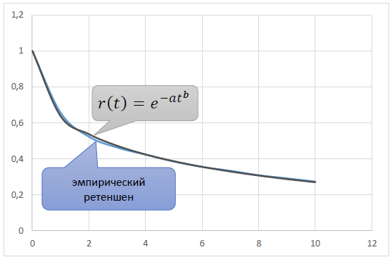
By selecting the parameters a and b, based on the requirement of the proximity of the theoretical r(t) to the empirical retention, it is possible to obtain a model curve that accurately reflects the real:

Accordingly, the same law L'(t) applies to the LTV curve=Ce^{−at b}, which, when integrated, gives the formula:

Formula **By selecting a, b and C, it is also possible to obtain a model LTV curve close to the actual one. The problem has been solved, and in conclusion, we can give a few small additional comments.

The first remark: about the power trend

Property 3), meaning the finiteness of the audience for r(t) and the finiteness of LTV for L(t) is fulfilled only at β > -1, that is, at b > 0.

If we consider the same model p(t) = at ^β at β = -1, we get:

r(t) = Ct^−α is a power function that cannot take the value r(0) = 1 and is not integrable at infinity at α < 1, but at such α the model corresponds to it:

The latter is a power function, the same “power trend” that marketers often use to approximate the LTV curve.

Conclusion. The power trend for the LTV curve, although it does not satisfy, unlike the model (**), conditions 1) and 3), is still its marginal special case for b → -1 with simultaneous a → ∞ . And since marketers use a “power trend” and consider it relevant to the behavior of the LTV curve, then a more general model (**) can even more be considered relevant.

Second remark: about increasing the number of parameters

If the analyst has a large amount of statistical data, he may want to fit the approximation curve closer to them, in the hope that it will give more accurate forecasts in this case.

At the same time, he is ready to allow more additional parameters into the model. For example, to build r(t) not two-parameter, like our model (*), but three-, four- or five-parameter.

How can this wish be satisfied while remaining within the framework of the constructed model?

It is possible to simulate mixtures of players. For example, we assume that our traffic consists of a mixture of two varieties of users with weights p and 1−p, and each variety has its own parameters – a ₁, b ₁ and a ₂,b ₂, respectively. Then it will work:

Similarly, you can increase the number of parameters in the LTV model:

If you need even more parameters, you can use mixtures of three or more “user varieties”.

However, it is necessary to involve multiparametric models with great caution. If there are a lot of parameters, then the analytical curve can adjust to random outliers, fluctuations in statistics and set trends that actually do not exist. In this case, of course, a multiparametric model will be closer to statistical data than a simple one, but the forecasts and other conclusions obtained from it will be less accurate.

Therefore, before using a five-parameter model, it makes sense to think carefully five times, and whether you need it.

Third remark: how to use

For the practical application of the found models, you need to be able to do two things. Take an integral of the form (**) and find the optimal set of parameters a, b, C.

This integral is not taken in elementary functions, but can be expressed by replacing variables through the Lower incomplete gamma function γ(s,x), which can be set, for example, in MS Excel, through the Gamma function and Gamma distribution implemented in it with the following formula: =EXP(GAMMANLOG(s))*(GAMMA.RASP(x,s,1,TRUE)).

You can find the optimal set of parameters in the same MS Excel. To do this, you can write out the target function from the point of view of the Least squares Method, that is, the sum of the squares of the deviations of the theoretical curve from the statistical data. And then adjust the parameters using the “Solution Search” add-in, selecting the “Search for solutions to nonlinear problems by the OPG method” method in it.

Thus, neither special software nor involvement of programmers is required to use the proposed models.

That’s it. I hope you were interested. If something has raised questions, be sure to unsubscribe in the comments.