One of the most important metrics of any shareware game is Lifetime Value (LTV), the total revenue of the game received from one client for all time. How to calculate it, – Isaac Roseboom, chief data analyst at DeltaDNA, told in his article. And our friends from SoftPressRelease translated his work into Russian.

Calculating the exact value of each installation is the most important component of F2P business planning. Especially if each installation can cost you $1-2. For this reason, many publishers devote significant resources to developing accurate LTV prediction methods. As a rule, these methods fall under one of three approaches:
- The “ARPDAU” model
- The “Transactions” model
- The “Players” model
In the first model, revenue is forecast by day. In the second – the number and amount of transactions for each player. And finally, the third model uses the historical value of players with the same demographic indicators. Next, we will not only explain in detail the calculation of each of these models, but also tell you when it would be more appropriate to apply one or another approach.
1) ARPDAU modeling: a simple approach
The most common approach is to use <ARPDAU> and <Retention> indicators to determine LTV. Mathematically, it looks like this:
LTV = <ARPDAU> X <Total days in the game>
The average number of days per installation is calculated from the retention curve by selecting a power function, i.e.:
R ∝ d – α
There are several options for selecting α, however, the simplest of them is using regression to select log (R) ∝ log(d). The use of linear regression is not recommended, since the errors of log(R) values do not have a normal distribution.
After determining the degree of slope of the power function, <Total days in the game> for d = D days after installation, is calculated from the integral of the power function of retention, i.e.:
<Total days in the game> =
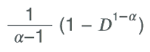
This value can then be used with ARPDAU to get LTV.
As a training example, let’s assume that ARPDAU = $0.1, and our hold from D1 to D7 is 35%, 28%, 25%, 21%, 18%, 15% and 13%. Power function selection gives α= 1,3, which in turn leads to <Total days in the game> = 2,77 days for D = 365 days.
This means that our LTV = $0.28.
This method of calculating the estimated LTV is, without a doubt, one of the simplest. However, for this simplicity, we have to put up with some disadvantages. Firstly, in the case of long-lived games, ARPDAU will be based on existing players who may be more inclined to buy than the group for which you are trying to build a forecast. In addition to this, the retention rate for all players is usually worse than for paying players in particular. Ultimately, this means that the typical error in forecasts using this method is 30 – 40%, for groups of 500 or more players.
2) Transaction modeling: Focus on those who pay
A more complex approach involves modeling the number of transactions that a player will make in his “life”.
You can construct a statistical model that will give P (T|D), i.e. the probability of a player making a transaction on the day after installing D. If Nt is the number of transactions observed on day = t, then on some future day = D, the estimated number of transactions will be:
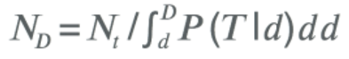
The conversion to payer can be modeled similarly, i.e. P (C|D) is the probability that the player will become a payer on day = D.
These probability distributions can be described by various “long-tail” distributions. Different distributions are suitable for different types of games. For example, power functions are usually well suited for PC games, and gamma distribution is good for social casino games.
These models can be compiled using numerical methods. The libraries in R and Python allow you to do this with ease. In R, the fitdistr function allows you to match a set of probability distributions with a data set by numerically searching for maximum likelihood parameters. After obtaining the best distribution for the models, LTV per day = D can be calculated as

Where <T> is the average value of an in-game purchase, ND is the estimated number of transactions per day = D, and CD is the estimated number of conversions per day = D.
The advantage of this approach is that it models the behavior of players generating LTV, that is, payers. Accurate conversion modeling is paramount for games that convert a lot of players at late stages, for example, MMO. Transaction modeling is important for games with a high number of transactions per payer, i.e., for casual puzzles or other games without premium currency.
Although this method assumes greater accuracy than the first one, it is still based on working with groups, therefore it requires an adequate amount of players to achieve accuracy, i.e. it cannot give you a good method for calculating the LTV of an individual user.
If this limitation is not taken into account, provided that suitable distributions and testing are used, this type of model, as a rule, reaches about 20% accuracy (for groups of 500 or more players).
3) Player simulation: prediction of individual LTV
The ideal option would be to be able to make a reliable assessment of the LTV of each individual player. This would not only allow for acquisition and profitability decisions, but would also change the way games interact with players, for example, players with low LTV would receive more advertising, and players with high LTV would receive VIP offers.
To predict LTV at the player level, it is necessary to use more detailed information about the player, including demographic and behavioral data. Example of the type of metrics that can be used: country, device type, frequency of gaming sessions, success rate, number of in-game friends, etc.
Using data sets for different time intervals, these metrics can be used when building a regression model to calculate LTV. Depending on the underlying metric distributions, a single model may be used, or players may be segmented into different groups with different characteristics, for example, it may be necessary to use completely different regression models for players on iOS and Android.
The compiled models can be used to predict the LTV of individual players. The LTV of a group can be found by taking the average of the individual assumed LTVs.
All these functions can be performed using statistical packages in R or Python. In R, kmeans or hclust can be used for data segmentation, and glm can be used for regression.
The obvious advantage of this approach is to obtain an individual LTV. For the reliability of the result, however, extensive, relevant data over a long period of time is needed. This means that this method cannot be used during the launch of a new game or after significant game updates.
Making accurate models
Although all three LTV models can show good results, the answer to the question of which model to use depends on the situation in which your game is located. If you have a small number of players with a relatively short “life” (for example, a few weeks), then model 1 is best for you).
If you have a significant number of players, and you expect a large spread in “life” and cost structures depending on the group, then model 2 is needed).
Finally, if you have a well-established game with a stable version and loyal players, Model 3) can offer significant advantages.
In any case, the most important point is to test your models on data from past time periods in order to verify their accuracy and understand their limitations. Finally, we note that under no circumstances is it possible to make plausible LTV models from too small a sample (for example, <100 players). In such cases, an approximate method like LTV = 4 x ARPDAU is more likely to give you a better understanding than any of the statistical approaches.
Source: DeltaDNA Translation: