Matchup: Reverse Balance Engineering (Part 1)

0. About the subject of the article

When developing and releasing the game, we inevitably rely on the experience of other teams and other projects in every aspect — from the design of the gameplay (flappy bird rules!) before choosing an attraction strategy (for example, high virality = low Acquisition Cost, vivat Candy Crush).

The mathematical model regulating the game complexity and managing the economic cycles in the game is no exception. In an attempt to create the perfect balance within your game, one of the key success factors is a detailed analysis of similar successful projects, which allows you to understand their mathematical essence — a set of laws governing the game economy and gameplay. Such laws can then be used in your project, adapting them, if necessary, to the realities of your game. The process of identifying these mathematical laws is what we call reverse engineering (from the words “engineering” — i.e. design, and “reverse” — i.e. reverse).

In this article, we will try to figure out exactly what reverse engineering is, how this process works, what we have to operate as a result of this process and what its fruits are.

As always, the article is not a specific guide to action and does not contain precise laws, but simply reflects our personal experience in this matter and our approaches to understanding and implementing reverse engineering.

1. About formulas and numbers

Imagine two variables, one of which depends on the other. For example, the symbol E denotes the amount of experience that a player needs to earn to move to the next level, and the symbol x indicates the current level of the player. Let E depend on x (i.e., for example, being at the first level, the player needs to gain 10 experience to move to the next, second, level, and being at the fifth level — 100 experience to move to the next, sixth).

The dependence of E on x is usually written in the form of E(x) and it is said that E is a function of the argument x (therefore, E is written in uppercase, and x is lowercase). Such dependence can be presented in two forms:

• Continuous, using the equation (for example, E(x) = x2);
• Discrete, using a table (each specific value of x will correspond to the value of E).

The main difference between a continuous form and a discrete one is the following: if a function is given continuously, its value can be obtained for any argument value (of course, if for this argument value the function value is computable in principle). But what does it mean for us?

Having a tabular task of the function in your hands, you know its value only for the argument values selected in advance (in our example, these are the values of x = 1, 2, 3, 4, 5 If you have an equation in your hands, you will be able to determine the value of the function not only for the same x = 1, 2, 3, 4, 5, etc., but also for any others — for example, for x = -2 or x = 3.75. In our example with level and experience, the values x = -2 or x = 3.75 do not make sense (because the level is a positive integer!), but think about it: that is, your tablet ends at the value x = 100, and you needed to find out how much experience a player must gain to move from 101 to 102 levels? In order to answer this question, an equation will be required.

Initially, analyzing another (someone else’s) project, you get only a discrete record for each function available in the game. Imagine that when making a farm, you took as a basis the balance of a popular game in this genre, began to gain one level after another and write out how much experience it would take to get the next level. After passing a hundred levels, you will get a discrete record of the function E(x) — a table in which there will be a hundred lines, one for each integer value of x starting from 1.

You will have a lot of questions about this entry. For example: what will be the value of E for x = 150? by what principle are these numbers chosen? how fast do they increase with increasing x? does the growth rate of these numbers increase or decrease?

This is how we approach the main tasks of reverse engineering. Reverse engineering of the project’s mathematics is designed primarily to identify dependencies in the game, and secondly, to obtain a continuous record of these dependencies. Identifying dependencies will allow us to understand which of the game variables are related to each other. Obtaining a continuous record (i.e. an equation) will give us the opportunity to use these dependencies at our discretion, as well as modify them to suit our needs.

2. Sampling, approximation and other staff

The process of transition from continuous recording to discrete recording, it must be understood, is quite simple. Having an equation in your hands, you can consistently substitute various values of the argument into it and get the corresponding values of the function. In our example, substituting x = 1, 2, 3, 4, 5 and so on. in the equation E(x) = x2, we get the values for E = 1, 4, 9, 16, 25 etc. This process is called function discretization.

The reverse process (obtaining an equation from a table of values), called approximation, is usually much more complicated. It is he who is of particular interest to us. Before discussing how we will approximate, let’s understand why exactly this is necessary.

Using the correct terminology, it is possible to designate the following tasks that the approximation allows you to perform:

• Interpolation, i.e. getting intermediate values of a function (remember the example about finding E for x = 2.5, which doesn’t make much sense in the case of levels, but when calculating other functions it can become a headache if we only have a tabular record of the function);
• Extrapolation, i.e. getting values outside the initially described area (this task needs to be solved if the table ended at x = 100, and you need to find E for x = 150).
• Analysis, i.e. obtaining information about the behavior of the function (in other words, getting a picture of what is happening). For example, what can we say about the growth of experience “to the next level”, having the formula E(x) = x2 in hand? The obvious conclusion is that E increases with the growth of x, i.e. for a higher level it takes more experience to move to the next one. A less obvious conclusion is that the growth rate of E is not only positive, but also increases. This means that the further the player has advanced, the greater the percentage of experience required for the next level increases. After receiving the function, as part of its analysis, it will also be possible to compare it with other functions in order to understand which of them grow faster, which are slower, and thereby see how the game balance changes for the player over time.

3. Identifying dependencies

Our first task, even before the approximation makes sense, is to identify those dependencies whose continuous recording we would like to obtain. As a rule, game cycles are built on a variety of different dependencies, simple and not so.

In our example, the dependence of E on x is revealed “by eye”. For a game in the “farm” genre, the amount of experience needed to move to the next level is unlikely to depend on the character’s current equipment or the number of his friends.

Basically, when analyzing a project, you will encounter more complex dependencies. The approach to their identification can be represented by the following set of steps:

• To form a primary list of game variables that may depend on others (for our example, the purchase price of a product in a store may depend on its level or characteristics; or everything is more complicated — the characteristics may depend on its level, and the price on the characteristics);
• To form a primary list of game variables that most likely do not depend on anything, or the law of their formation is extremely clear (for example, the number of the next level is always +1 from the previous one, and the reward for a new level is always +1 coin);
• Make a list of all dependencies that are potentially possible (for example, the price of an item from its level, the price of an item from its parameters, its level from its parameters, etc.);
• Conduct an initial study of these potential dependencies to see if they look like dependencies or look like random sets of numbers.

When compiling a list of potential dependencies for research, it is important not to be afraid to start. The key to fearlessness is simple: you need to remember that if the selected dependency does not turn out to be a dependency at all, its analysis will show you to understand it, and you can safely exclude this dependency from your list.

Let’s focus in more detail on the item “initial research”, which, in theory, should cause the most concern. Let’s take an example: let’s say in the game under study you need to grow plants and sell them in your store. Plants become available for cultivation at different levels, have different maturation times and are sold by the player for different amounts of coins. Various dependency options are possible here: the sale price and maturation time may depend on the level at which these plants become available, or they may depend on each other.

In the described case, I would start with a parallel analysis of both options. Imagine that there are only 10 plants in the game. The data for each of them is described in the table below.

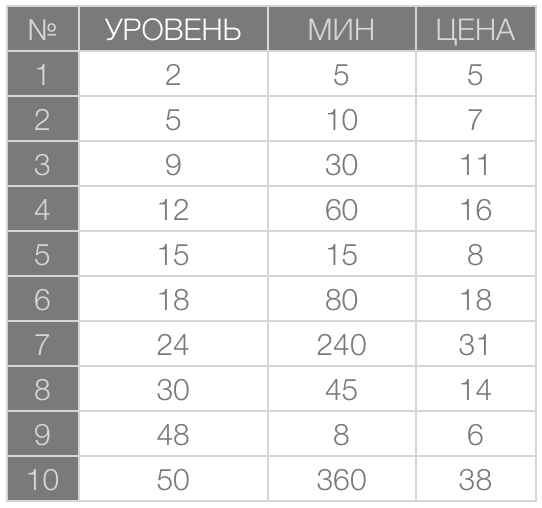
Here, in the left column, each plant is assigned an ordinal number (instead of a name). The following columns for each plant show the level of its availability to the player, the ripening time in minutes and the sale price to the store.

Let ‘s try to analyze the following dependencies:

• Time from level;
• The price depends on the time.

You will laugh, but I think the most practical way to identify a dependency is to plot a proposed function based on its tabular record. It’s easy to build such graphs. We select two columns of the table, sort them in ascending order of the values in the argument column, and then put the values in the argument column on the x axis, and the values in the function column on the y axis.

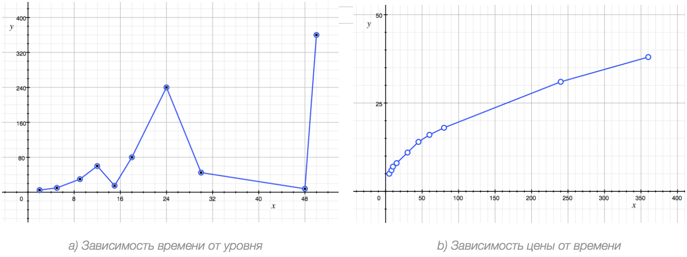
That’s what we got. In the variant on the left, the values in the MIN column act as a function, and the values in the LEVEL column act as an argument. For the option on the right, the function is the PRICE, and the argument is represented by the MIN column.

There are many ways to approximate the tabular record of certain types of equations, but, as I said, in practice, the most convenient is to observe the constructed graph. In order to understand whether the resulting graph is a representation of a function, and not a random set of points, look at it and ask yourself a simple question: can I mentally (at least theoretically) continue the graph further? We see that in case a) this is hardly possible (here we have a polyline that goes up and down, and we will not be able to predict its behavior). Whereas in case b) it is obvious to us that the chart will go up further, and its growth rate will slow down. This means that in the case of a) we are dealing with the absence of dependence, and in the case of b) — with its presence.

Before rushing to approximate functions and make full use of graphs, one more thing needs to be noticed. Let me make a prediction: even if you masterfully approximate a set of values, the resulting function will never reproduce tabular data one hundred percent accurately. This happens for two reasons:

• Rounding. The formula used by the balance developer in one case or another does not care about the beauty of the numbers given to it. So the square root of two is a number with an infinite number of decimal places. It is impossible to put such a number in the game, so you have to round it up. Note that on small numbers, rounding makes a particularly large spread in the data. For example, the same root of two, which is equal to 1.4142135… I can round it up to 1.5, and if there should be only integers in the game, then to 1 or 2. The difference by one in this case is very significant. For example, the numbers 100 and 101 that differ by one are essentially only 1% different, whereas 1 and 2 differ by 100%!
• Manual “tuning” is a special headache with reverse engineering. Often (and this is correct) the developer uses the formula he uses only as a starting point, i.e. with its help he builds only the primary version of the balance, which he then rules with his hands in some places, based on criteria such as his personal flair, game statistics, player wishes, etc. Being manually configured, the numbers may not just deviate from the formula a little, but significantly confuse the one who is trying to identify the original law. To demonstrate, let’s look at a simple example.

Let’s say we found out that by level 18 a player begins to experience significant difficulties with the game (for example, he does not have enough game money), because of this he gets tired of playing and leaves, never to return. We solved the problem simply — for a plant that is issued at level 18 (ordinal number 6 in our table), we artificially increased the sale price to 50 so that the player would receive a powerful mechanism for making money and experience a surge of strength (such an example, of course, is exaggerated, but for the purposes of demostration it is quite similar).

Below are two charts — the initial one and the one that we will get after such a manual balance adjustment.

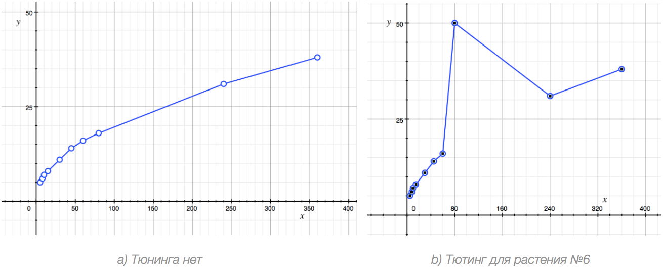
The graph on the right clearly shows a point away from the general law. In this case (and in general, always), the most useful thing, in order not to lose the big picture, will be to exclude such points from consideration. If we remove the point (80, 50) on the graph on the right and connect the neighboring points of the line, we will see the graph of the function almost as clearly as on the left.

The main recommendations may sound like this: do not let individual numbers deceive you and do not be afraid of peaks that are far from the general law. If possible, exclude them from consideration in order to return to their justification later.

4. All sorts of different types of functions

So, we have a tabular distribution, according to which we have already built a graph. We can mentally continue this graph, thereby gaining an understanding of what a function is in front of us. As I said, there are many mathematical methods of approximation, but, as practice shows, we should be interested in some natural algorithm that will allow us not to lose understanding of what exactly we are doing.

The first step in such an algorithm is to understand what type of function the graph of which we see. The type of function defines the basic form of its graph, which we can then modify (shift, compress, stretch) using scaling coefficients (i.e., any numerical terms and multipliers that we enter into the equation).

There are many different types of functions. Some are so complex that you will never guess from their graph that this is an equation, and not a random set of points. Fortunately, in 99% of cases we do not deal with such functions. Below I will try to list the most used types of functions and show how their graphs look like. After studying this section, you should have no problems in order to determine the type of function by the appearance of the graph.

In the future, for simplicity, we will use the following entry:

• The function argument will be denoted by the letter x;
• The value of the function will be denoted by the letter y;
• The entry y = f(x) will mean that the variable y is represented by some equation, where x acts as an argument;
• The letters a, b, c, etc. will denote constants, i.e. some numbers that are included in the equation f(x) and do not depend on x.

4.1. Constant function

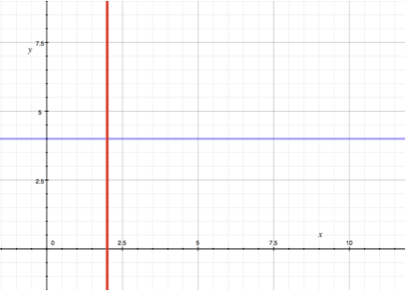
This is the simplest example. In the equation of such a function, x and y actually do not depend on each other at all!

Examples: y = 4, x = 2.

The graph on the left shows two functions. The blue one is described by the equation y = a (here the function y takes the value a for any x), and the red one is described by the equation x = b (here the argument is fixed in the value b, and y takes any values).

In fact, if y = a, it means that y does not change, no matter what the argument x is. For example, if we said that the amount of replenished energy of a player per minute is 1, and it does not matter what level the player has, this is an example of a constant function.

4.2. Linear function

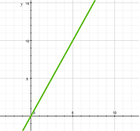
Such a function is generally described by the equation y = a*x + b.

Examples: y = x, y= 2*x + 3, y = 5-x.

The graph of such a function is a straight line inclined at some angle to the axes. The picture shows the function y = 2*x, its graph passes through the origin (because the value of the function at x = 0 is also 0). In general, this line does not have to pass through the origin.

The main feature of the linear function is a constant rate of growth (or decrease in the case of a < 0). Imagine that the selling price of a plant linearly depends on the time of its production. In this case, it can be shown that if plant A ripens twice as long as B, then it will cost twice as much. Simple laws are advantageous to set by a linear function because of its simplicity. For example, saying that the maximum amount of energy a player has is a level multiplied by one-third, and rounding it down to an integer each time, we get a simple law: every three levels, the maximum amount of energy increases by 1.

4.3. Power function

This type of function contains several subtypes, which in practice it is convenient to consider separately. Each of these subtypes is represented by the same formula: y = k*xa + b, but differs from the others by the interval in which the number a lies.

a = 1, a = 0

As you might guess, a linear function and a constant function are special cases of a power function. In the case of a = 1 we are dealing with a linear function (y = k*x + b), and in the case of a = 0 — with a constant (y = k + b).

a > 1

In this case, the graph of the function is a curve called a parabola.

Examples: y = x3, y = 4*x3+3.

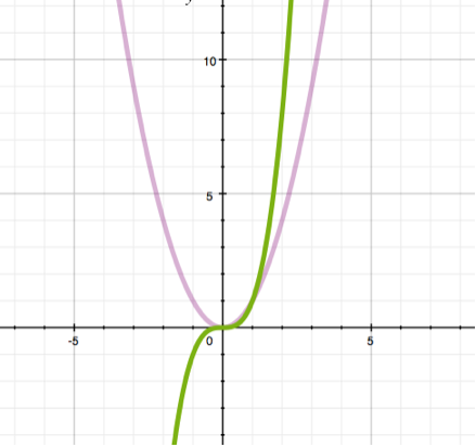
The graph above shows the functions y = x2 (purple curve) and y = x3 (green curve). As a rule, we will be interested exclusively in the upper right quarter of the coordinate space (where y and x are positive), however, it is necessary to understand the difference in the behavior of functions of this type and on other quarters. Note that the cubic parabola (green) goes down when x becomes less than zero and continues to decrease, while the square parabola (purple) increases on the same segment. In fact, any parabola where a is even will never take a negative value (because negative x, when raised to an even power, will give a positive result), while parabolas with odd powers can take negative values (for example, -3, raised to a cube, will give -9).

The peculiarity of such a function is that it allows you to organize growth at an increasing rate. As a rule, such functions are applied to an increase in game complexity, requirements for the player or an increase in the deficit. An obvious example that we have already considered earlier is the increase in the amount of experience required to reach the next level. Often developers use a degree of 2 or 3 to set this growth. Another example is an increase in the time of growing plants, depending on the level. Here, if the unlock level of plant A is twice as high as that of plant B, then its production time will be more than twice the production time of B.

0 < a < 1

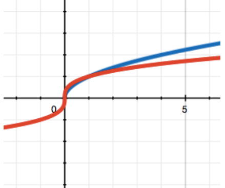
The graph of such a function is similar to a parabola rotated by 90 degrees.

Examples: y = √x, y= 2* x1/3.

The graph shows the square (blue) and cubic (red) roots of x. Note again that on x < 0 the functions behave differently. There, the square root of a negative number is not defined at all, but the cubic one exists.

It is necessary to understand that the root of x is still a power function. This can be clearly demonstrated by the example of a square and a square root. So the “x-square” is x to the power of 2, and the “square root of x” is x to the power of 1/2. Each time the power of x can be represented by a fraction in which the numerator is the power of x and the denominator is the power of the root of x. So x to the power of 2/3 is essentially the cubic root of x squared.

Note that the value of the degree itself determines the growth rate of the function. In the case of a > 1 — the larger a is, the faster the function grows (see graph to resp. the point at which the cube grows faster than the square). Here the situation is exactly the same: 1/2 is greater than 1/3, so the square root of x will grow faster than the cubic one.

Functions of this type are needed when we want to slow down the game progress. Look at our example with a table of selling prices of plants depending on the time of their maturation. The selling price increases with time, but this growth slows down. The graph obtained from the table is very similar in shape to the root, isn’t it?

a < 0

To understand the meaning of the negative degree is quite simple. It only says that the argument is in the denominator. So, for example, the entry y = x-3 means the same thing as the entry y = 1/x3.

The graph of a function of this type is called a hyperbola.

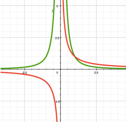
The graph shows the functions for a = -1 (red) and a = -2 (green). Again, notice the differences in the behavior of functions on different parts of the coordinate space. The function for a = -1 exists in two opposite quarters (i.e. the sign y will either always coincide with x, or always be opposite, depending on the constants included in the formula), but in the case of a = -2, the function exists in one half (the sign y will either always be positive or always negative, depending on the constants in the formula).

You can use such a function in order to organize the decrease of some value in the game. Note that the rate of such a decrease will decrease over time.

Generalization

Power functions are most often used in game design. They are easily amenable to research and allow you to organize the increase or decrease of a particular value with a well-defined speed, the change of which is also easy to control. All subtypes of power functions are closely related to each other. So, for example, finding that y is equal to x squared, you can safely state (at least in a positive quarter of space) that x is equal to the root of y.

There is a more general form for a power function — the so-called polynomial of degree n. It is written in this form: y = kn * xn + kn-1 * xn-1 + kn-2 * xn-2 + … + k0 * x0. For example, a polynomial of degree 4 is y = 2*x4+ 1*x3 + x1 + 3. Here k2 = 0, so we do not meet the term x2.

In practice, the use of such a function is justified, because it allows for more precise and fine-tuning of the balance (in fact, this formula has more “levers” that can be twisted to adjust the balance in one direction or another), however, this function is more difficult to study and requires more detailed mathematical apparatus for tuning.

4.4. Exponential function

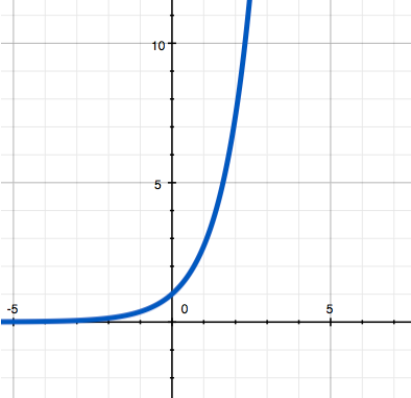
This function can be written as y = k * ax. The argument here no longer acts as the basis of the degree (i.e., what is raised to a degree), but its indicator (i.e., a number showing to what degree we are raising). The base is a constant.

A striking example, shown in the graph on the left, is the popular “exponent” function, which we used to consider the business card of the balance of Asian MMORPGs. The exponent is y = ex, where e is a famous special number with a number of remarkable mathematical properties. It is approximately equal to 2.718281828 (it is easy to remember — the numbers 2 and 7 are followed twice by the year of birth of Leo Tolstoy =).

The graph of such a function looks like a parabola, but increases (or decreases if a is less than one) much faster. For small a (for example, 1.000000001), the exponential function will increase more slowly, but sooner or later it will still overtake any power function.

The exponential function is used if they want to organize a very sharp increase in any value (in Asian MMOs, this function is used to increase the amount of experience needed to reach the next level in order to organize a rapid slowdown in the player’s progress through the levels).

4.5. Logarithmic function

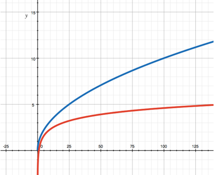
I don’t often use the logarithmic function in calculations, but that won’t stop me from mentioning it in the article. Suddenly faced with it in the balance of the game we are analyzing, we should be ready to learn this function as well.

The logarithm with the base a of the number x is the degree to which you need to raise a to get x. Thus, writing the expression y = logax is like saying that ay = x.

From this definition it follows that the logarithmic function is the inverse of the exponential, i.e. if we know that y is the logarithm of the base a of x, then we can get the inverse law: x is a to the power of y.

In the figure, the logarithm along the base e (red) is shown in comparison with the square root (blue). The most commonly used are logarithms with bases 2 (binary), e (linear) and 10 (decimal), while the larger the base of the logarithm, the higher its graph will be. Note that if the base a < 1, then the logarithmic function decreases.

4.6. Trigonometric functions sin and cos

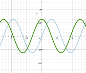
They are also rarely used when designing game balance, but it would be somehow disrespectful not to mention them here.

The figure shows the graphs y = sin(x) (blue) and y = cos(x) (green). Their characteristic feature is periodicity. You can use them if you want to organize the periodicity and repeatability in the game. For example, if there are seasons in your game, then the yield (or the happiness of the nation) can change according to a similar law (increases in summer and falls in winter).

As follows from the above, a logarithmic function arises if two variables are connected by an exponential law. This law is too harsh, and in most cases it is rarely suitable as a basis for building a game balance. However, it makes sense if you want to “sharply tighten the nuts” at later stages of the game, in order, for example, to stretch the time for which the player will exhaust all the remaining content and leave before the next update of the game. As far as I remember, Blizzard often did this with its World of Warcraft back at the dawn of its existence.

You will find the conclusions and conclusion in the second part of the article.